Compute Many Estimates and Errors in Just a Single Shot

Computes many estimates and errors (e.g. for disparate estimation domains) in just a single shot, primarily to use them in fitting GVF models. Can handle estimators of all kinds.

svystat(design, kind = c("TM", "R", "S", "SR", "B", "Q", "L", "Sigma", "Sigma2"),
        by = NULL, group = NULL, forGVF = TRUE,
        combo = -1, ...)

# S3 method for gvf.input.gr
plot(x, ...)

# S3 method for svystat.gr
coef(object, ...)
# S3 method for svystat.gr
SE(object, ...)
# S3 method for svystat.gr
VAR(object, ...)
# S3 method for svystat.gr
cv(object, ...)
# S3 method for svystat.gr
deff(object, ...)
# S3 method for svystat.gr
confint(object, ...)

Arguments

design	Object of class `analytic` (or inheriting from it) containing survey data and sampling design metadata.
kind	`character` specifying the summary statistics function to call: it may be `'TM'` (i.e. `svystatTM`, the default), `'R'` (i.e. `svystatR`), `'S'` (i.e. `svystatS`), `'SR'` (i.e. `svystatSR`), `'B'` (i.e. `svystatB`), `'Q'` (i.e. `svystatQ`), `'L'` (i.e. `svystatL`), `'Sigma'` (i.e. `svySigma`), and `'Sigma2'` (i.e. `svySigma2`).
by	Formula specifying the variables that define the "estimation domains". If `NULL` (the default option) estimates refer to the whole population.
group	Formula specifying a partition of the population into "groups": the output will be returned separately for each group. If `NULL` (the default option) the output is returned as a whole.
forGVF	Select `TRUE` (the default) if you want to use the output to fit a GVF model. Otherwise, the output will be simply a set of summary statistics objects.
combo	An `integer` which is only meaningful if `by` is passed. Requests to compute outputs for all the domains determined by crossing the `by` variables up to a given order (see ‘Details’).
...	For function `svystat`, additional arguments to the summary statistic function implied by `kind`. Otherwise, further arguments passed to or from other methods.
x	The object of class `gvf.input.gr` to plot.
object	An object of class `svystat.gr` containing survey statistics.

Details

This function can compute all the summary statistics provided by ReGenesees, and is principally meant to return a lot of them in just a single shot.

If forGVF = TRUE the output will be ready to feed ReGenesees GVF fitting infrastructure, otherwise it will consist simply of a set of summary statistic objects.

Use argument kind to specify the summary statistic you need. The default value 'TM' selects function svystatTM, which yields Totals and Means. All the arguments needed by the summary statistic function implied by kind (e.g. argument y for svystatTM when kind = 'TM') will be passed on through argument ‘...’.

As usual in summary statistics, argument by can be used to request domain estimates.

The group formula (if any) specifies a way of partitioning the population into groups: the output will be reported separately for each group. In the GVF context, a “grouped” output will permit to fit separate GVF models inside different groups (and hence to compute separate variance predictions for different groups).

Note that group and by share identical syntax and semantics as model formulae, despite they have different purposes in function svystat (as explained above).

Parameter combo is only meaningful if by is passed. Its purpose is to allow computing estimates and errors simultaneously for many estimation domains.

If the by formula involves n variables, specifying combo = m requests to compute outputs for all the domains determined by all the interactions of by variables up to order m (with -1 <= m <= n), as follows:

  COMBO         MEANING
  m = -1.......'no combo', i.e. treat 'by' formula as usual (the default);
  m =  0.......'order zero' combination, i.e. just a single domain:
                the whole population;
  m =  1.......'order zero' plus 'order one' combinations, the latter being
                all the marginal domains defined by 'by' variables;
  m =  n........combinations of any order, the maximum being the one with
                all 'by' variables interacting simultaneously.

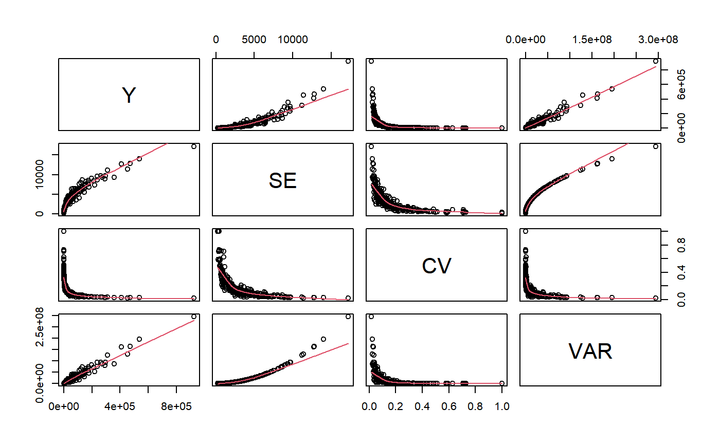
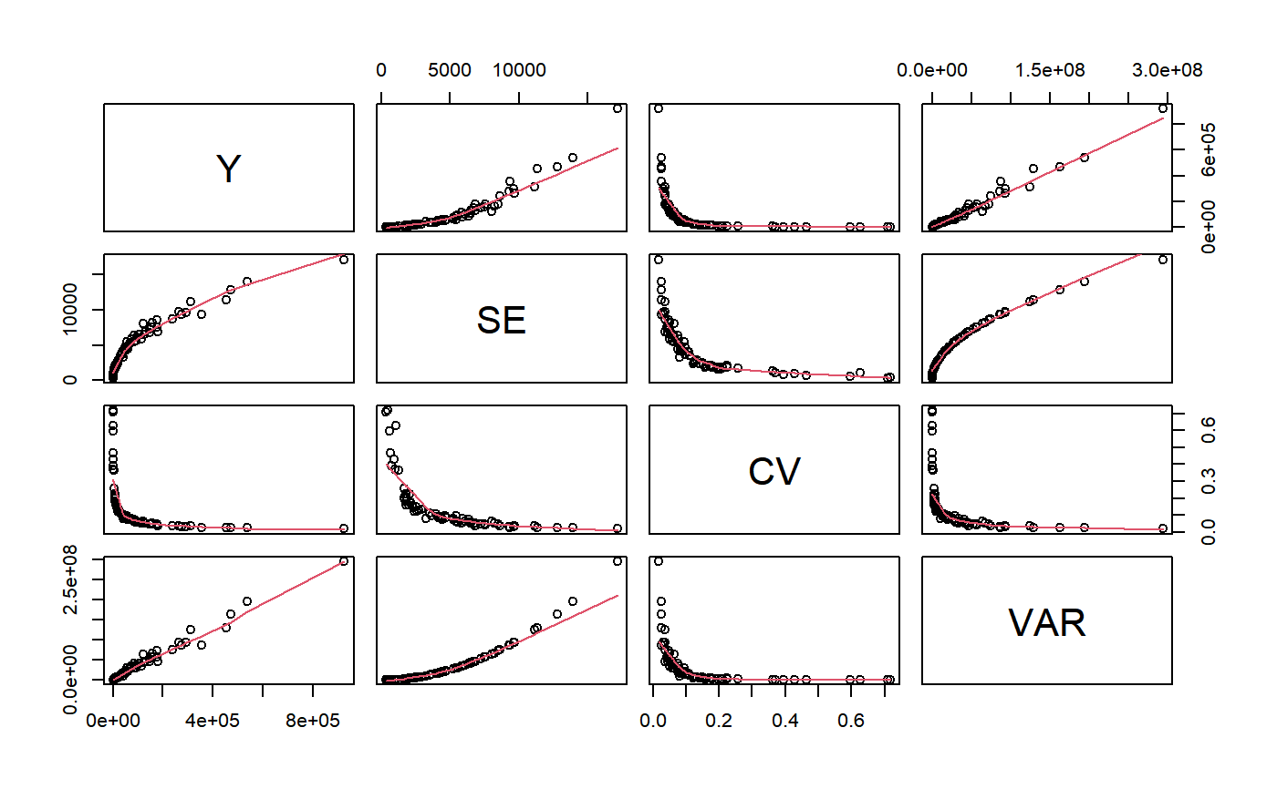
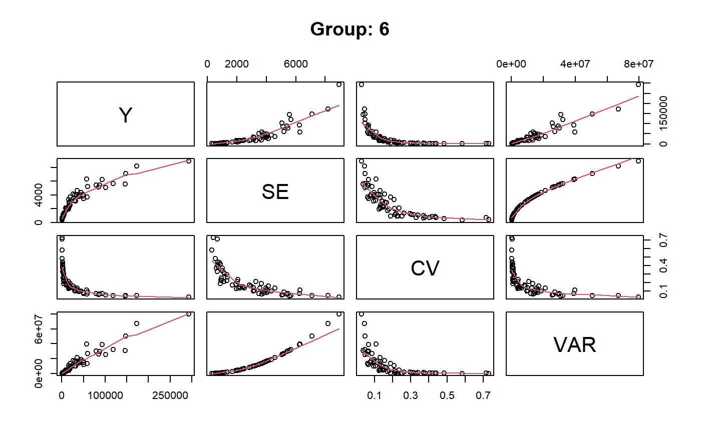
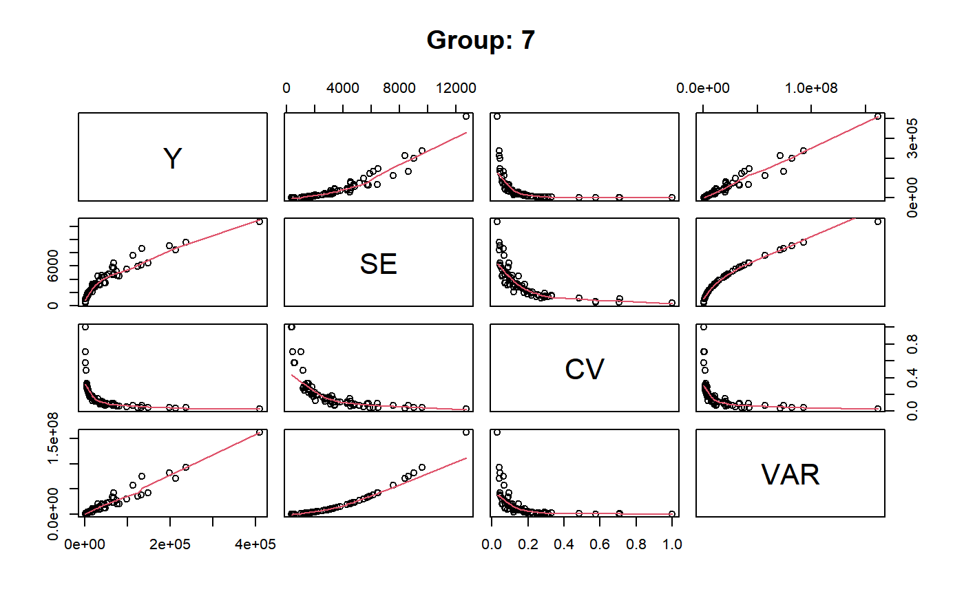
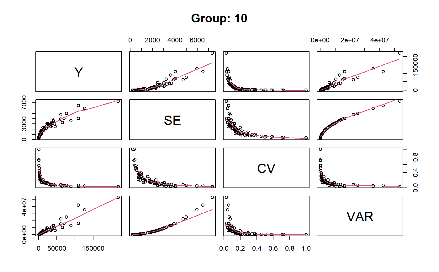
The plot method can be used only when forGVF = TRUE and produces a matrix (or many matrices, if group is passed) of scatterplots with polynomial smoothers.

Methods coef, SE, VAR, cv, deff, and confint can be used only when forGVF = FALSE, to extract estimates and variability statistics.

Value

An object storing estimates and errors, whose detailed structure depends on input parameters' values.

If forGVF = FALSE, a set of summary statistics possibly stored into a list (with class svystat.gr in the most general case).

If forGVF = TRUE and argument group is not passed, an object of class gvf.input.

If forGVF = TRUE and argument group is passed, an object of class gvf.input.gr. This is a list of objects of class gvf.input, each one pertaining to a different population group.

Examples

# Load sbs data:
data(sbs)

# Create a design object:
sbsdes<-e.svydesign(data=sbs,ids=~id,strata=~strata,weights=~weight,fpc=~fpc)


##########################################################################
# svystat as an alternative way to compute 'ordinary' summary statistics #
##########################################################################
## Total number of employees
svystat(sbsdes,y=~emp.num,forGVF=FALSE)
#>            Total       SE
#> emp.num 985157.9 1421.315
# equivalent to:
svystatTM(sbsdes,y=~emp.num)
#>            Total       SE
#> emp.num 985157.9 1421.315

## Average number of employees per enterprise
svystat(sbsdes,y=~emp.num,estimator="Mean",forGVF=FALSE)
#>             Mean         SE
#> emp.num 56.88635 0.08207154
# equivalent to:
svystatTM(sbsdes,y=~emp.num,estimator="Mean")
#>             Mean         SE
#> emp.num 56.88635 0.08207154

## Average value added per employee by economic activity macro-sector
## (nace.macro):
svystat(sbsdes,kind="R",num=~va.imp2,den=~emp.num,by=~nace.macro,forGVF=FALSE)
#>              nace.macro va.imp2/emp.num SE.va.imp2/emp.num
#> Agriculture Agriculture        58.59297          3.2226705
#> Industry       Industry        47.93647          0.6580034
#> Commerce       Commerce       226.99062         12.9021106
#> Services       Services        36.89123          0.5767339
# equivalent to:
svystatR(sbsdes,num=~va.imp2,den=~emp.num,by=~nace.macro)
#>              nace.macro va.imp2/emp.num SE.va.imp2/emp.num
#> Agriculture Agriculture        58.59297          3.2226705
#> Industry       Industry        47.93647          0.6580034
#> Commerce       Commerce       226.99062         12.9021106
#> Services       Services        36.89123          0.5767339

## Counts of employees by classes of number of employees (emp.cl) crossed
## with economic activity macro-sector (nace.macro):
svystat(sbsdes,y=~emp.num,by=~emp.cl:nace.macro,forGVF=FALSE)
#>                        emp.cl  nace.macro Total.emp.num SE.Total.emp.num
#> [6,9].Agriculture       [6,9] Agriculture      731.3167         9.281259
#> (9,19].Agriculture     (9,19] Agriculture     2624.4359        44.575649
#> (19,49].Agriculture   (19,49] Agriculture     2922.5615        68.861432
#> (49,99].Agriculture   (49,99] Agriculture     1999.6154        47.694076
#> (99,Inf].Agriculture (99,Inf] Agriculture     8761.0000         0.000000
#> [6,9].Industry          [6,9]    Industry    15427.1899       104.285002
#> (9,19].Industry        (9,19]    Industry    31917.7212       243.654881
#> (19,49].Industry      (19,49]    Industry    69637.7435       749.906901
#> (49,99].Industry      (49,99]    Industry    84114.6819       785.184314
#> (99,Inf].Industry    (99,Inf]    Industry   380357.0000         0.000000
#> [6,9].Commerce          [6,9]    Commerce     9909.9941       131.532367
#> (9,19].Commerce        (9,19]    Commerce    12319.5145       213.766128
#> (19,49].Commerce      (19,49]    Commerce    13644.2736       488.404994
#> (49,99].Commerce      (49,99]    Commerce     8177.2696       248.297022
#> (99,Inf].Commerce    (99,Inf]    Commerce    25166.0000         0.000000
#> [6,9].Services          [6,9]    Services    11994.3642        88.687559
#> (9,19].Services        (9,19]    Services    15626.5388       165.977429
#> (19,49].Services      (19,49]    Services    21886.4967       379.537665
#> (49,99].Services      (49,99]    Services    23109.1340       468.271619
#> (99,Inf].Services    (99,Inf]    Services   244831.0000         0.000000
# equivalent to:
svystatTM(sbsdes,y=~emp.num,by=~emp.cl:nace.macro)
#>                        emp.cl  nace.macro Total.emp.num SE.Total.emp.num
#> [6,9].Agriculture       [6,9] Agriculture      731.3167         9.281259
#> (9,19].Agriculture     (9,19] Agriculture     2624.4359        44.575649
#> (19,49].Agriculture   (19,49] Agriculture     2922.5615        68.861432
#> (49,99].Agriculture   (49,99] Agriculture     1999.6154        47.694076
#> (99,Inf].Agriculture (99,Inf] Agriculture     8761.0000         0.000000
#> [6,9].Industry          [6,9]    Industry    15427.1899       104.285002
#> (9,19].Industry        (9,19]    Industry    31917.7212       243.654881
#> (19,49].Industry      (19,49]    Industry    69637.7435       749.906901
#> (49,99].Industry      (49,99]    Industry    84114.6819       785.184314
#> (99,Inf].Industry    (99,Inf]    Industry   380357.0000         0.000000
#> [6,9].Commerce          [6,9]    Commerce     9909.9941       131.532367
#> (9,19].Commerce        (9,19]    Commerce    12319.5145       213.766128
#> (19,49].Commerce      (19,49]    Commerce    13644.2736       488.404994
#> (49,99].Commerce      (49,99]    Commerce     8177.2696       248.297022
#> (99,Inf].Commerce    (99,Inf]    Commerce    25166.0000         0.000000
#> [6,9].Services          [6,9]    Services    11994.3642        88.687559
#> (9,19].Services        (9,19]    Services    15626.5388       165.977429
#> (19,49].Services      (19,49]    Services    21886.4967       379.537665
#> (49,99].Services      (49,99]    Services    23109.1340       468.271619
#> (99,Inf].Services    (99,Inf]    Services   244831.0000         0.000000

## Provided forGVF = FALSE, you can use estimator.kind on svystat output:
stat<-svystat(sbsdes,kind="R",num=~va.imp2,den=~emp.num,by=~emp.cl:nace.macro,
      group=~region,forGVF=FALSE)
stat
#> $North
#>                            region   emp.cl  nace.macro va.imp2/emp.num
#> North.[6,9].Agriculture     North    [6,9] Agriculture       366.96371
#> North.(9,19].Agriculture    North   (9,19] Agriculture       125.14796
#> North.(19,49].Agriculture   North  (19,49] Agriculture        26.38628
#> North.(49,99].Agriculture   North  (49,99] Agriculture        40.69757
#> North.(99,Inf].Agriculture  North (99,Inf] Agriculture        40.78901
#> North.[6,9].Industry        North    [6,9]    Industry       149.44154
#> North.(9,19].Industry       North   (9,19]    Industry        93.67811
#> North.(19,49].Industry      North  (19,49]    Industry        71.30895
#> North.(49,99].Industry      North  (49,99]    Industry        54.98881
#> North.(99,Inf].Industry     North (99,Inf]    Industry        42.17408
#> North.[6,9].Commerce        North    [6,9]    Commerce       284.44988
#> North.(9,19].Commerce       North   (9,19]    Commerce       285.75077
#> North.(19,49].Commerce      North  (19,49]    Commerce       343.19045
#> North.(49,99].Commerce      North  (49,99]    Commerce       277.32682
#> North.(99,Inf].Commerce     North (99,Inf]    Commerce       119.01810
#> North.[6,9].Services        North    [6,9]    Services       114.79726
#> North.(9,19].Services       North   (9,19]    Services       108.58072
#> North.(19,49].Services      North  (19,49]    Services        81.84604
#> North.(49,99].Services      North  (49,99]    Services        49.24988
#> North.(99,Inf].Services     North (99,Inf]    Services        23.62823
#>                            SE.va.imp2/emp.num
#> North.[6,9].Agriculture             69.399164
#> North.(9,19].Agriculture            23.521324
#> North.(19,49].Agriculture            7.379092
#> North.(49,99].Agriculture            6.878927
#> North.(99,Inf].Agriculture           0.000000
#> North.[6,9].Industry                10.542207
#> North.(9,19].Industry                6.876373
#> North.(19,49].Industry               4.276559
#> North.(49,99].Industry               4.406634
#> North.(99,Inf].Industry              0.000000
#> North.[6,9].Commerce                53.520240
#> North.(9,19].Commerce               33.649105
#> North.(19,49].Commerce              65.511219
#> North.(49,99].Commerce              41.975198
#> North.(99,Inf].Commerce              0.000000
#> North.[6,9].Services                12.025794
#> North.(9,19].Services                7.641878
#> North.(19,49].Services               5.870567
#> North.(49,99].Services               3.834554
#> North.(99,Inf].Services              0.000000
#> 
#> $Center
#>                             region   emp.cl  nace.macro va.imp2/emp.num
#> Center.[6,9].Agriculture    Center    [6,9] Agriculture       255.17000
#> Center.(9,19].Agriculture   Center   (9,19] Agriculture        77.44690
#> Center.(19,49].Agriculture  Center  (19,49] Agriculture        54.65256
#> Center.(49,99].Agriculture  Center  (49,99] Agriculture        28.89706
#> Center.(99,Inf].Agriculture Center (99,Inf] Agriculture        71.19741
#> Center.[6,9].Industry       Center    [6,9]    Industry        59.87445
#> Center.(9,19].Industry      Center   (9,19]    Industry        34.18783
#> Center.(19,49].Industry     Center  (19,49]    Industry        65.88804
#> Center.(49,99].Industry     Center  (49,99]    Industry        26.98472
#> Center.(99,Inf].Industry    Center (99,Inf]    Industry        29.40858
#> Center.[6,9].Commerce       Center    [6,9]    Commerce       250.78978
#> Center.(9,19].Commerce      Center   (9,19]    Commerce       352.27161
#> Center.(19,49].Commerce     Center  (19,49]    Commerce       177.15472
#> Center.(49,99].Commerce     Center  (49,99]    Commerce       209.69909
#> Center.(99,Inf].Commerce    Center (99,Inf]    Commerce        75.61189
#> Center.[6,9].Services       Center    [6,9]    Services       225.47039
#> Center.(9,19].Services      Center   (9,19]    Services        72.56336
#> Center.(19,49].Services     Center  (19,49]    Services        81.61965
#> Center.(49,99].Services     Center  (49,99]    Services        32.95646
#> Center.(99,Inf].Services    Center (99,Inf]    Services        27.64846
#>                             SE.va.imp2/emp.num
#> Center.[6,9].Agriculture            134.721936
#> Center.(9,19].Agriculture            35.177421
#> Center.(19,49].Agriculture           12.999974
#> Center.(49,99].Agriculture           10.348290
#> Center.(99,Inf].Agriculture           0.000000
#> Center.[6,9].Industry                11.869080
#> Center.(9,19].Industry                4.301401
#> Center.(19,49].Industry               9.918660
#> Center.(49,99].Industry               2.081170
#> Center.(99,Inf].Industry              0.000000
#> Center.[6,9].Commerce                37.069887
#> Center.(9,19].Commerce               87.846914
#> Center.(19,49].Commerce              28.297146
#> Center.(49,99].Commerce              55.335978
#> Center.(99,Inf].Commerce              0.000000
#> Center.[6,9].Services                19.646717
#> Center.(9,19].Services               10.978079
#> Center.(19,49].Services               9.053992
#> Center.(49,99].Services               2.193392
#> Center.(99,Inf].Services              0.000000
#> 
#> $South
#>                            region   emp.cl  nace.macro va.imp2/emp.num
#> South.[6,9].Agriculture     South    [6,9] Agriculture      184.591520
#> South.(9,19].Agriculture    South   (9,19] Agriculture       40.105422
#> South.(19,49].Agriculture   South  (19,49] Agriculture       34.953927
#> South.(99,Inf].Agriculture  South (99,Inf] Agriculture        2.538631
#> South.[6,9].Industry        South    [6,9]    Industry      114.786806
#> South.(9,19].Industry       South   (9,19]    Industry       87.405151
#> South.(19,49].Industry      South  (19,49]    Industry       51.414112
#> South.(49,99].Industry      South  (49,99]    Industry       57.637797
#> South.(99,Inf].Industry     South (99,Inf]    Industry       45.439600
#> South.[6,9].Commerce        South    [6,9]    Commerce      469.637600
#> South.(9,19].Commerce       South   (9,19]    Commerce      218.753010
#> South.(19,49].Commerce      South  (19,49]    Commerce      237.570888
#> South.(49,99].Commerce      South  (49,99]    Commerce       65.432565
#> South.(99,Inf].Commerce     South (99,Inf]    Commerce      159.420290
#> South.[6,9].Services        South    [6,9]    Services       58.804592
#> South.(9,19].Services       South   (9,19]    Services      106.823712
#> South.(19,49].Services      South  (19,49]    Services       59.160541
#> South.(49,99].Services      South  (49,99]    Services       47.408801
#> South.(99,Inf].Services     South (99,Inf]    Services       22.027478
#>                            SE.va.imp2/emp.num
#> South.[6,9].Agriculture            40.8041969
#> South.(9,19].Agriculture            9.9078878
#> South.(19,49].Agriculture           8.3784352
#> South.(99,Inf].Agriculture          0.0000000
#> South.[6,9].Industry               13.6388730
#> South.(9,19].Industry              13.1573725
#> South.(19,49].Industry              4.8598330
#> South.(49,99].Industry              4.3907101
#> South.(99,Inf].Industry             0.0000000
#> South.[6,9].Commerce              157.2612126
#> South.(9,19].Commerce              42.4770659
#> South.(19,49].Commerce             39.7773417
#> South.(49,99].Commerce             31.5943961
#> South.(99,Inf].Commerce             0.0000000
#> South.[6,9].Services                9.6455143
#> South.(9,19].Services              15.6861187
#> South.(19,49].Services              4.1040128
#> South.(49,99].Services              0.9976743
#> South.(99,Inf].Services             0.0000000
#> 
#> attr(,"group.vars")
#> [1] "region"
#> attr(,"class")
#> [1] "svystat.gr" "list"      
estimator.kind(stat,sbsdes)
#> [1] "Ratio"


##########################################################
# Understanding syntax and semantics of argument 'combo' #
##########################################################
# Load household data:
data(data.examples)

# Create a design object:
houdes<-e.svydesign(data=example,ids=~towcod+famcod,strata=~SUPERSTRATUM,
        weights=~weight)

# Add convenience variable 'ones' to estimate counts:
houdes<-des.addvars(houdes,ones=1)

## To facilitate understanding, let's for the moment keep forGVF = FALSE.
## Let's use estimates and errors of counts of individuals by sex and
## five age classes (age5c):
svystat(houdes,y=~ones,by=~age5c:sex,forGVF=FALSE)
#>     age5c sex Total.ones SE.Total.ones
#> 1.f     1   f    70394.0      5272.598
#> 2.f     2   f   147004.4      7237.907
#> 3.f     3   f   177780.1      7547.864
#> 4.f     4   f    65782.8      5235.777
#> 5.f     5   f     9099.5      2043.608
#> 1.m     1   m    58534.4      4475.785
#> 2.m     2   m   147570.7      6700.508
#> 3.m     3   m   178683.8      6829.000
#> 4.m     4   m    57114.8      5425.453
#> 5.m     5   m    12136.8      1970.159

## Now let's play with argument 'combo':
   # combo = -1
   # -> 'no combo', i.e. treat 'by' formula as usual
   svystat(houdes,y=~ones,by=~age5c:sex,forGVF=FALSE,combo=-1)
#>     age5c sex Total.ones SE.Total.ones
#> 1.f     1   f    70394.0      5272.598
#> 2.f     2   f   147004.4      7237.907
#> 3.f     3   f   177780.1      7547.864
#> 4.f     4   f    65782.8      5235.777
#> 5.f     5   f     9099.5      2043.608
#> 1.m     1   m    58534.4      4475.785
#> 2.m     2   m   147570.7      6700.508
#> 3.m     3   m   178683.8      6829.000
#> 4.m     4   m    57114.8      5425.453
#> 5.m     5   m    12136.8      1970.159

   # combo = 0
   # -> 'order zero' combination, i.e. just a single domain: the whole population
   svystat(houdes,y=~ones,by=~age5c:sex,forGVF=FALSE,combo=0)
#>         Total       SE
#> ones 924101.3 17172.68

   # combo = 1
   # -> 'order zero' plus 'order one' combinations, the latter being all the
   #    marginal domains defined by 'by' variables
   svystat(houdes,y=~ones,by=~age5c:sex,forGVF=FALSE,combo=1)
#> $population
#>         Total       SE
#> ones 924101.3 17172.68
#> 
#> $age5c
#>   age5c Total.ones SE.Total.ones
#> 1     1   128928.4      6855.457
#> 2     2   294575.1      9646.795
#> 3     3   356463.9      9354.653
#> 4     4   122897.6      8022.848
#> 5     5    21236.3      2728.266
#> 
#> $sex
#>   sex Total.ones SE.Total.ones
#> f   f   470060.8      12796.39
#> m   m   454040.5      11359.58
#> 
#> attr(,"class")
#> [1] "svystat.gr" "list"      

   # combo = 2
   # -> since 'by' has 2 variables, this means combinations of any order up to
   #    the maximum
   svystat(houdes,y=~ones,by=~age5c:sex,forGVF=FALSE,combo=2)
#> $population
#>         Total       SE
#> ones 924101.3 17172.68
#> 
#> $age5c
#>   age5c Total.ones SE.Total.ones
#> 1     1   128928.4      6855.457
#> 2     2   294575.1      9646.795
#> 3     3   356463.9      9354.653
#> 4     4   122897.6      8022.848
#> 5     5    21236.3      2728.266
#> 
#> $sex
#>   sex Total.ones SE.Total.ones
#> f   f   470060.8      12796.39
#> m   m   454040.5      11359.58
#> 
#> $`age5c:sex`
#>     age5c sex Total.ones SE.Total.ones
#> 1.f     1   f    70394.0      5272.598
#> 2.f     2   f   147004.4      7237.907
#> 3.f     3   f   177780.1      7547.864
#> 4.f     4   f    65782.8      5235.777
#> 5.f     5   f     9099.5      2043.608
#> 1.m     1   m    58534.4      4475.785
#> 2.m     2   m   147570.7      6700.508
#> 3.m     3   m   178683.8      6829.000
#> 4.m     4   m    57114.8      5425.453
#> 5.m     5   m    12136.8      1970.159
#> 
#> attr(,"class")
#> [1] "svystat.gr" "list"      

   # combo = 3
   # -> yields an error, as 'combo' cannot exceed the number of 'by' variables
   #    (2 in this example)
if (FALSE) {
   svystat(houdes,y=~ones,by=~age5c:sex,forGVF=FALSE,combo=3)
}


######################################################################
# svystat as an alternative way to prepare input data for GVF models #
######################################################################
## The same estimates and errors of the last example above, now with
## forGVF = TRUE: note the different output data format
svystat(houdes,y=~ones,by=~age5c:sex,combo=2)
#>        name        Y        SE         CV       VAR
#> 1      ones 924101.3 17172.681 0.01858312 294900983
#> 2    1:ones 128928.4  6855.457 0.05317259  46997295
#> 3    2:ones 294575.1  9646.795 0.03274817  93060661
#> 4    3:ones 356463.9  9354.653 0.02624292  87509530
#> 5    4:ones 122897.6  8022.848 0.06528075  64366083
#> 6    5:ones  21236.3  2728.266 0.12847181   7443435
#> 7    f:ones 470060.8 12796.386 0.02722283 163747492
#> 8    m:ones 454040.5 11359.582 0.02501887 129040102
#> 9  1.f:ones  70394.0  5272.598 0.07490124  27800288
#> 10 2.f:ones 147004.4  7237.907 0.04923599  52387294
#> 11 3.f:ones 177780.1  7547.864 0.04245618  56970252
#> 12 4.f:ones  65782.8  5235.777 0.07959188  27413358
#> 13 5.f:ones   9099.5  2043.608 0.22458468   4176335
#> 14 1.m:ones  58534.4  4475.785 0.07646418  20032649
#> 15 2.m:ones 147570.7  6700.508 0.04540541  44896804
#> 16 3.m:ones 178683.8  6829.000 0.03821835  46635241
#> 17 4.m:ones  57114.8  5425.453 0.09499207  29435544
#> 18 5.m:ones  12136.8  1970.159 0.16232937   3881527

## Note that the agile command above is indeed equivalent to the following
## lengthier, cumbersome statement:
gvf.input(houdes,
          svystatTM(houdes,y=~ones),
          svystatTM(houdes,y=~ones,by=~age5c),
          svystatTM(houdes,y=~ones,by=~sex),
          svystatTM(houdes,y=~ones,by=~age5c:sex)
          )
#>        name        Y        SE         CV       VAR
#> 1      ones 924101.3 17172.681 0.01858312 294900983
#> 2    1:ones 128928.4  6855.457 0.05317259  46997295
#> 3    2:ones 294575.1  9646.795 0.03274817  93060661
#> 4    3:ones 356463.9  9354.653 0.02624292  87509530
#> 5    4:ones 122897.6  8022.848 0.06528075  64366083
#> 6    5:ones  21236.3  2728.266 0.12847181   7443435
#> 7    f:ones 470060.8 12796.386 0.02722283 163747492
#> 8    m:ones 454040.5 11359.582 0.02501887 129040102
#> 9  1.f:ones  70394.0  5272.598 0.07490124  27800288
#> 10 2.f:ones 147004.4  7237.907 0.04923599  52387294
#> 11 3.f:ones 177780.1  7547.864 0.04245618  56970252
#> 12 4.f:ones  65782.8  5235.777 0.07959188  27413358
#> 13 5.f:ones   9099.5  2043.608 0.22458468   4176335
#> 14 1.m:ones  58534.4  4475.785 0.07646418  20032649
#> 15 2.m:ones 147570.7  6700.508 0.04540541  44896804
#> 16 3.m:ones 178683.8  6829.000 0.03821835  46635241
#> 17 4.m:ones  57114.8  5425.453 0.09499207  29435544
#> 18 5.m:ones  12136.8  1970.159 0.16232937   3881527


  ################################################
  # Using argument 'group' to prepare input data #
  # for separate GVF models                      #
  ################################################
  ## The same estimates and errors of the last example above, now prepared
  ## separately for different regions (regcod):
  svystat(houdes,y=~ones,by=~age5c:sex,combo=2,group=~regcod)
#> $`6`
#>          name        Y        SE         CV        VAR
#> 1      6:ones 293458.3 8923.8062 0.03040911 79634317.2
#> 2    6.1:ones  40903.4 4080.2341 0.09975293 16648310.2
#> 3    6.2:ones  93387.9 6248.6896 0.06691113 39046122.2
#> 4    6.3:ones 118888.1 5682.2007 0.04779453 32287404.5
#> 5    6.4:ones  34964.4 4605.3581 0.13171563 21209322.9
#> 6    6.5:ones   5314.5 1131.0289 0.21281943  1279226.3
#> 7    6.f:ones 147487.3 7115.8574 0.04824726 50635427.1
#> 8    6.m:ones 145971.0 5566.5674 0.03813475 30986672.6
#> 9  6.1.f:ones  22115.0 3131.3939 0.14159593  9805627.9
#> 10 6.2.f:ones  44476.2 4337.1112 0.09751533 18810533.4
#> 11 6.3.f:ones  59710.2 5198.9486 0.08706969 27029066.3
#> 12 6.4.f:ones  19465.0 3663.7726 0.18822361 13423230.0
#> 13 6.5.f:ones   1720.9  695.4733 0.40413348   483683.1
#> 14 6.1.m:ones  18788.4 2531.7660 0.13475155  6409839.0
#> 15 6.2.m:ones  48911.7 4059.2074 0.08299052 16477164.9
#> 16 6.3.m:ones  59177.9 3694.3741 0.06242827 13648400.3
#> 17 6.4.m:ones  15499.4 1970.9812 0.12716500  3884767.0
#> 18 6.5.m:ones   3593.6 1131.3951 0.31483612  1280054.8
#> 
#> $`7`
#>          name        Y        SE         CV       VAR
#> 1      7:ones 410671.9 12714.366 0.03095991 161655092
#> 2    7.1:ones  55833.8  4814.445 0.08622815  23178885
#> 3    7.2:ones 131681.4  6148.902 0.04669529  37808992
#> 4    7.3:ones 148350.1  6489.953 0.04374754  42119485
#> 5    7.4:ones  63302.5  5796.072 0.09156150  33594447
#> 6    7.5:ones  11504.1  2216.158 0.19264069   4911355
#> 7    7.f:ones 212537.3  8415.166 0.03959383  70815025
#> 8    7.m:ones 198134.6  9038.617 0.04561857  81696591
#> 9  7.1.f:ones  31771.0  3604.749 0.11346036  12994216
#> 10 7.2.f:ones  66546.2  4784.696 0.07190036  22893313
#> 11 7.3.f:ones  74654.8  4559.773 0.06107809  20791527
#> 12 7.4.f:ones  33306.9  3255.533 0.09774349  10598493
#> 13 7.5.f:ones   6258.4  1834.256 0.29308703   3364495
#> 14 7.1.m:ones  24062.8  3107.262 0.12913135   9655076
#> 15 7.2.m:ones  65135.2  4724.222 0.07252947  22318271
#> 16 7.3.m:ones  73695.3  5181.339 0.07030759  26846270
#> 17 7.4.m:ones  29995.6  4500.199 0.15002863  20251789
#> 18 7.5.m:ones   5245.7  1294.904 0.24685051   1676776
#> 
#> $`10`
#>           name        Y        SE         CV        VAR
#> 1      10:ones 219971.1 7321.9925 0.03328616 53611573.6
#> 2    10.1:ones  32191.2 2677.7042 0.08318125  7170100.0
#> 3    10.2:ones  69505.8 4025.6113 0.05791763 16205546.6
#> 4    10.3:ones  89225.7 3619.7569 0.04056855 13102640.3
#> 5    10.4:ones  24630.7 3092.2990 0.12554653  9562313.4
#> 6    10.5:ones   4417.7 1119.3094 0.25336928  1252853.6
#> 7    10.f:ones 110036.2 6503.6175 0.05910434 42297040.1
#> 8    10.m:ones 109934.9 4044.3589 0.03678867 16356838.9
#> 9  10.1.f:ones  16508.0 2236.1673 0.13545961  5000444.1
#> 10 10.2.f:ones  35982.0 3268.5544 0.09083860 10683447.6
#> 11 10.3.f:ones  43415.1 3024.8402 0.06967254  9149658.4
#> 12 10.4.f:ones  13010.9 1841.6391 0.14154587  3391634.7
#> 13 10.5.f:ones   1120.2  572.8502 0.51138207   328157.3
#> 14 10.1.m:ones  15683.2 1991.9172 0.12700961  3967734.0
#> 15 10.2.m:ones  33523.8 2470.0948 0.07368183  6101368.3
#> 16 10.3.m:ones  45810.6 2478.0174 0.05409266  6140570.4
#> 17 10.4.m:ones  11619.8 2301.9531 0.19810609  5298988.3
#> 18 10.5.m:ones   3297.5  961.6113 0.29161829   924696.3
#> 
#> attr(,"group.vars")
#> [1] "regcod"
#> attr(,"class")
#> [1] "gvf.input.gr" "list"        

  ## Again the same estimates and errors, prepared separately for groups
  ## defined crossing marital status (marstat) and region:
  svystat(houdes,y=~ones,by=~age5c:sex,combo=2,group=~marstat:regcod)
#> $married.6
#>                  name        Y        SE         CV        VAR
#> 1      married.6:ones 173001.9 8183.3890 0.04730231 66967855.7
#> 2    married.6.1:ones   5967.7 1315.6942 0.22046922  1731051.1
#> 3    married.6.2:ones  57155.1 6302.4072 0.11026850 39720336.2
#> 4    married.6.3:ones  79175.5 5469.7271 0.06908358 29917914.3
#> 5    married.6.4:ones  26504.1 4136.7694 0.15608036 17112860.9
#> 6    married.6.5:ones   4199.5  944.2243 0.22484207   891559.4
#> 7    married.6.f:ones  87840.2 5409.9384 0.06158841 29267433.1
#> 8    married.6.m:ones  85161.7 5118.0128 0.06009759 26194054.6
#> 9  married.6.1.f:ones   4077.5  937.6069 0.22994651   879106.7
#> 10 married.6.2.f:ones  27145.1 3565.8442 0.13136235 12715244.5
#> 11 married.6.3.f:ones  39672.3 3781.5369 0.09531933 14300021.1
#> 12 married.6.4.f:ones  15802.5 3308.0005 0.20933400 10942867.2
#> 13 married.6.5.f:ones   1142.8  553.0390 0.48393336   305852.2
#> 14 married.6.1.m:ones   1890.2  823.5977 0.43571988   678313.2
#> 15 married.6.2.m:ones  30010.0 3966.9579 0.13218787 15736754.7
#> 16 married.6.3.m:ones  39503.2 3919.4184 0.09921775 15361840.8
#> 17 married.6.4.m:ones  10701.6 1943.2926 0.18158898  3776386.3
#> 18 married.6.5.m:ones   3056.7 1038.0655 0.33960332  1077579.9
#> 
#> $unmarried.6
#>                    name        Y        SE         CV        VAR
#> 1      unmarried.6:ones 101776.7 5053.8683 0.04965644 25541584.6
#> 2    unmarried.6.1:ones  33965.7 4046.9080 0.11914690 16377464.6
#> 3    unmarried.6.2:ones  32410.4 3122.1231 0.09633090  9747652.6
#> 4    unmarried.6.3:ones  30093.6 3199.6627 0.10632369 10237841.3
#> 5    unmarried.6.4:ones   4728.9  896.3779 0.18955316   803493.4
#> 6    unmarried.6.5:ones    578.1  421.7000 0.72945865   177830.9
#> 7    unmarried.6.f:ones  50867.3 3495.6179 0.06872033 12219344.4
#> 8    unmarried.6.m:ones  50909.4 3830.8081 0.07524756 14675091.1
#> 9  unmarried.6.1.f:ones  17067.5 2873.2550 0.16834657  8255594.4
#> 10 unmarried.6.2.f:ones  15640.3 2373.0681 0.15172779  5631452.2
#> 11 unmarried.6.3.f:ones  15591.7 2101.6684 0.13479405  4417010.0
#> 12 unmarried.6.4.f:ones   1989.7  755.2217 0.37956562   570359.8
#> 13 unmarried.6.5.f:ones    578.1  421.7000 0.72945865   177830.9
#> 14 unmarried.6.1.m:ones  16898.2 2450.0347 0.14498791  6002670.0
#> 15 unmarried.6.2.m:ones  16770.1 2213.2098 0.13197356  4898297.5
#> 16 unmarried.6.3.m:ones  14501.9 2202.0284 0.15184413  4848928.9
#> 17 unmarried.6.4.m:ones   2739.2 1015.0497 0.37056430  1030326.0
#> 
#> $widowed.6
#>                  name       Y        SE        CV        VAR
#> 1      widowed.6:ones 18679.7 2963.9010 0.1586696 8784709.00
#> 2    widowed.6.1:ones   970.0  694.1545 0.7156232  481850.50
#> 3    widowed.6.2:ones  3822.4 1169.1801 0.3058759 1366982.16
#> 4    widowed.6.3:ones  9619.0 2031.4324 0.2111896 4126717.63
#> 5    widowed.6.4:ones  3731.4  945.5378 0.2534003  894041.78
#> 6    widowed.6.5:ones   536.9  313.7392 0.5843532   98432.29
#> 7    widowed.6.f:ones  8779.8 2070.0963 0.2357794 4285298.53
#> 8    widowed.6.m:ones  9899.9 1697.3512 0.1714514 2881001.19
#> 9  widowed.6.1.f:ones   970.0  694.1545 0.7156232  481850.50
#> 10 widowed.6.2.f:ones  1690.8  626.5500 0.3705642  392564.90
#> 11 widowed.6.3.f:ones  4446.2 1318.1870 0.2964750 1737616.96
#> 12 widowed.6.4.f:ones  1672.8  734.4694 0.4390659  539445.31
#> 13 widowed.6.2.m:ones  2131.6  890.0968 0.4175722  792272.32
#> 14 widowed.6.3.m:ones  5172.8 1359.7397 0.2628634 1848892.02
#> 15 widowed.6.4.m:ones  2058.6  681.9549 0.3312712  465062.51
#> 16 widowed.6.5.m:ones   536.9  313.7392 0.5843532   98432.29
#> 
#> $married.7
#>                  name        Y       SE         CV      VAR
#> 1      married.7:ones 236734.3 9621.808 0.04064391 92579192
#> 2    married.7.1:ones   8804.0 1744.489 0.19814733  3043242
#> 3    married.7.2:ones  79792.2 4518.514 0.05662852 20416972
#> 4    married.7.3:ones  98530.9 5471.113 0.05552687 29933072
#> 5    married.7.4:ones  40925.0 4314.561 0.10542605 18615438
#> 6    married.7.5:ones   8682.2 1867.809 0.21513081  3488709
#> 7    married.7.f:ones 124346.9 5930.148 0.04769036 35166656
#> 8    married.7.m:ones 112387.4 7571.344 0.06736826 57325248
#> 9  married.7.1.f:ones   4636.9 1357.586 0.29277873  1843039
#> 10 married.7.2.f:ones  44528.6 3436.932 0.07718482 11812500
#> 11 married.7.3.f:ones  48107.9 3420.255 0.07109549 11698143
#> 12 married.7.4.f:ones  22683.2 2748.955 0.12118902  7556752
#> 13 married.7.5.f:ones   4390.3 1460.518 0.33266928  2133113
#> 14 married.7.1.m:ones   4167.1 1209.003 0.29013066  1461689
#> 15 married.7.2.m:ones  35263.6 3134.083 0.08887587  9822476
#> 16 married.7.3.m:ones  50423.0 4597.055 0.09116980 21132911
#> 17 married.7.4.m:ones  18241.8 3054.249 0.16743135  9328438
#> 18 married.7.5.m:ones   4291.9 1174.801 0.27372504  1380156
#> 
#> $unmarried.7
#>                    name        Y       SE         CV        VAR
#> 1      unmarried.7:ones 133872.4 8619.082 0.06438281 74288573.8
#> 2    unmarried.7.1:ones  46036.5 4315.928 0.09375014 18627235.8
#> 3    unmarried.7.2:ones  41122.7 4302.361 0.10462253 18510308.3
#> 4    unmarried.7.3:ones  34531.2 3825.310 0.11077838 14632998.7
#> 5    unmarried.7.4:ones  11768.2 2252.209 0.19138095  5072446.6
#> 6    unmarried.7.5:ones    413.8  413.800 1.00000000   171230.4
#> 7    unmarried.7.f:ones  67003.8 6437.437 0.09607570 41440592.8
#> 8    unmarried.7.m:ones  66868.6 5722.640 0.08558038 32748607.2
#> 9  unmarried.7.1.f:ones  26491.5 3182.758 0.12014261 10129948.8
#> 10 unmarried.7.2.f:ones  17819.6 2765.313 0.15518376  7646953.7
#> 11 unmarried.7.3.f:ones  17587.6 3213.184 0.18269597 10324548.6
#> 12 unmarried.7.4.f:ones   4691.3 1402.580 0.29897471  1967230.9
#> 13 unmarried.7.5.f:ones    413.8  413.800 1.00000000   171230.4
#> 14 unmarried.7.1.m:ones  19545.0 2762.214 0.14132588  7629828.2
#> 15 unmarried.7.2.m:ones  23303.1 3312.801 0.14216140 10974652.3
#> 16 unmarried.7.3.m:ones  16943.6 2078.289 0.12265923  4319284.7
#> 17 unmarried.7.4.m:ones   7076.9 1573.914 0.22240163  2477205.5
#> 
#> $widowed.7
#>                  name       Y        SE        CV        VAR
#> 1      widowed.7:ones 40065.2 4548.7671 0.1135341 20691282.2
#> 2    widowed.7.1:ones   993.3  573.5355 0.5774041   328943.0
#> 3    widowed.7.2:ones 10766.5 1916.2722 0.1779847  3672099.1
#> 4    widowed.7.3:ones 15288.0 2594.8146 0.1697288  6733062.6
#> 5    widowed.7.4:ones 10609.3 2137.7459 0.2014974  4569957.5
#> 6    widowed.7.5:ones  2408.1 1167.4542 0.4848031  1362949.4
#> 7    widowed.7.f:ones 21186.6 3148.4862 0.1486074  9912965.3
#> 8    widowed.7.m:ones 18878.6 2912.3930 0.1542695  8482033.3
#> 9  widowed.7.1.f:ones   642.6  453.8199 0.7062246   205952.5
#> 10 widowed.7.2.f:ones  4198.0 1318.9821 0.3141930  1739713.9
#> 11 widowed.7.3.f:ones  8959.3 2027.3541 0.2262849  4110164.7
#> 12 widowed.7.4.f:ones  5932.4 1569.2589 0.2645234  2462573.5
#> 13 widowed.7.5.f:ones  1454.3 1029.6366 0.7079946  1060151.4
#> 14 widowed.7.1.m:ones   350.7  350.7000 1.0000000   122990.5
#> 15 widowed.7.2.m:ones  6568.5 1668.0436 0.2539459  2782369.4
#> 16 widowed.7.3.m:ones  6328.7 1610.9163 0.2545414  2595051.2
#> 17 widowed.7.4.m:ones  4676.9 1557.4125 0.3330010  2425533.6
#> 18 widowed.7.5.m:ones   953.8  550.2708 0.5769247   302797.9
#> 
#> $married.10
#>                   name        Y        SE         CV        VAR
#> 1      married.10:ones 126944.0 5968.8444 0.04701951 35627104.0
#> 2    married.10.1:ones   4513.9  894.3470 0.19813177   799856.5
#> 3    married.10.2:ones  40674.5 3530.8468 0.08680738 12466879.1
#> 4    married.10.3:ones  61439.6 3890.1505 0.06331666 15133271.0
#> 5    married.10.4:ones  16956.8 2256.5625 0.13307715  5092074.5
#> 6    married.10.5:ones   3359.2  988.7783 0.29434935   977682.6
#> 7    married.10.f:ones  61382.5 4730.9097 0.07707261 22381506.3
#> 8    married.10.m:ones  65561.5 3221.6794 0.04913981 10379217.9
#> 9  married.10.1.f:ones   2672.6  757.6423 0.28348512   574021.9
#> 10 married.10.2.f:ones  21293.6 2531.1412 0.11886864  6406675.9
#> 11 married.10.3.f:ones  27295.2 2865.8517 0.10499471  8213106.0
#> 12 married.10.4.f:ones   9228.1 1716.0832 0.18596278  2944941.4
#> 13 married.10.5.f:ones    893.0  525.8683 0.58887831   276537.5
#> 14 married.10.1.m:ones   1841.3  717.3732 0.38960149   514624.4
#> 15 married.10.2.m:ones  19380.9 2201.5097 0.11359171  4846644.8
#> 16 married.10.3.m:ones  34144.4 2475.9041 0.07251274  6130101.0
#> 17 married.10.4.m:ones   7728.7 1723.0100 0.22293659  2968763.4
#> 18 married.10.5.m:ones   2466.2  837.3441 0.33952805   701145.1
#> 
#> $unmarried.10
#>                     name       Y        SE         CV        VAR
#> 1      unmarried.10:ones 77005.4 5018.0796 0.06516530 25181123.2
#> 2    unmarried.10.1:ones 26954.1 2617.4122 0.09710627  6850846.5
#> 3    unmarried.10.2:ones 23022.1 3033.8191 0.13177856  9204058.4
#> 4    unmarried.10.3:ones 21186.4 2166.0879 0.10223955  4691937.0
#> 5    unmarried.10.4:ones  5381.3 1578.6478 0.29335807  2492128.9
#> 6    unmarried.10.5:ones   461.5  327.1987 0.70898954   107059.0
#> 7    unmarried.10.f:ones 41270.0 3704.7516 0.08976864 13725184.2
#> 8    unmarried.10.m:ones 35735.4 2994.3930 0.08379346  8966389.3
#> 9  unmarried.10.1.f:ones 13359.8 1994.9978 0.14932842  3980016.4
#> 10 unmarried.10.2.f:ones 12320.2 1945.9428 0.15794734  3786693.5
#> 11 unmarried.10.3.f:ones 12777.2 1762.1482 0.13791349  3105166.3
#> 12 unmarried.10.4.f:ones  2812.8  968.4658 0.34430669   937926.1
#> 13 unmarried.10.1.m:ones 13594.3 1906.8274 0.14026668  3635990.7
#> 14 unmarried.10.2.m:ones 10701.9 1764.2318 0.16485220  3112513.7
#> 15 unmarried.10.3.m:ones  8409.2 1165.7427 0.13862706  1358956.1
#> 16 unmarried.10.4.m:ones  2568.5  982.4032 0.38248128   965116.0
#> 17 unmarried.10.5.m:ones   461.5  327.1987 0.70898954   107059.0
#> 
#> $widowed.10
#>                   name       Y        SE        CV        VAR
#> 1      widowed.10:ones 16021.7 2259.4330 0.1410233 5105037.66
#> 2    widowed.10.1:ones   723.2  418.5259 0.5787139  175163.94
#> 3    widowed.10.2:ones  5809.2 1234.0241 0.2124258 1522815.56
#> 4    widowed.10.3:ones  6599.7 1181.1396 0.1789687 1395090.76
#> 5    widowed.10.4:ones  2292.6  852.8892 0.3720183  727420.01
#> 6    widowed.10.5:ones   597.0  434.0183 0.7269988  188371.88
#> 7    widowed.10.f:ones  7383.7 1359.0597 0.1840622 1847043.27
#> 8    widowed.10.m:ones  8638.0 1351.2763 0.1564339 1825947.75
#> 9  widowed.10.1.f:ones   475.6  337.4288 0.7094802  113858.18
#> 10 widowed.10.2.f:ones  2368.2  734.2456 0.3100437  539116.59
#> 11 widowed.10.3.f:ones  3342.7  738.6556 0.2209757  545612.10
#> 12 widowed.10.4.f:ones   970.0  484.9514 0.4999499  235177.89
#> 13 widowed.10.5.f:ones   227.2  227.2000 1.0000000   51619.84
#> 14 widowed.10.1.m:ones   247.6  247.6000 1.0000000   61305.76
#> 15 widowed.10.2.m:ones  3441.0 1007.7442 0.2928638 1015548.38
#> 16 widowed.10.3.m:ones  3257.0  837.9413 0.2572740  702145.70
#> 17 widowed.10.4.m:ones  1322.6  599.8629 0.4535483  359835.54
#> 18 widowed.10.5.m:ones   369.8  369.8000 1.0000000  136752.04
#> 
#> attr(,"group.vars")
#> [1] "marstat" "regcod" 
#> attr(,"class")
#> [1] "gvf.input.gr" "list"        

  ## NOTE: Output has class "gvf.input.gr". This will tell ReGenesees' GVF
  ##       fitting facilities to handle estimates and errors pertaining to
  ##       different groups independently of each other.


## NOTE: Parameter combo allows svystat to gather a huge amount of estimates and
##       errors in just a single slot, as the number of estimation domains grows
##       exponentially with the number of by variables.
##       See, for instance, the following example:
out <- svystat(houdes,y=~ones,by=~age5c:marstat:sex:regcod,combo=4)
dim(out)
#> [1] 283   5
head(out)
#>     name        Y        SE         CV       VAR
#> 1   ones 924101.3 17172.681 0.01858312 294900983
#> 2 1:ones 128928.4  6855.457 0.05317259  46997295
#> 3 2:ones 294575.1  9646.795 0.03274817  93060661
#> 4 3:ones 356463.9  9354.653 0.02624292  87509530
#> 5 4:ones 122897.6  8022.848 0.06528075  64366083
#> 6 5:ones  21236.3  2728.266 0.12847181   7443435
plot(out)


##################################################
# Minor details: accessor functions and plotting #
##################################################
  ## Accessor functions work only when forGVF = FALSE
# Average value added per employee by nace.macro:
out <- svystat(sbsdes,kind="R",num=~va.imp2,den=~emp.num,by=~nace.macro,forGVF=FALSE)
out
#>              nace.macro va.imp2/emp.num SE.va.imp2/emp.num
#> Agriculture Agriculture        58.59297          3.2226705
#> Industry       Industry        47.93647          0.6580034
#> Commerce       Commerce       226.99062         12.9021106
#> Services       Services        36.89123          0.5767339
# Access CV values and confidence intervals:
cv(out)
#>             CV.va.imp2/emp.num
#> Agriculture         0.05500097
#> Industry            0.01372657
#> Commerce            0.05683984
#> Services            0.01563336
confint(out)
#>                                 2.5 %    97.5 %
#> Agriculture:va.imp2/emp.num  52.27665  64.90929
#> Industry:va.imp2/emp.num     46.64680  49.22613
#> Commerce:va.imp2/emp.num    201.70294 252.27829
#> Services:va.imp2/emp.num     35.76085  38.02161

# The same as above, separately for regions:
out <- svystat(sbsdes,kind="R",num=~va.imp2,den=~emp.num,by=~nace.macro,group=~region,forGVF=FALSE)
out
#> $North
#>                   region  nace.macro va.imp2/emp.num SE.va.imp2/emp.num
#> North.Agriculture  North Agriculture        60.73814          3.9277681
#> North.Industry     North    Industry        51.58483          0.8132740
#> North.Commerce     North    Commerce       220.89970         15.2905919
#> North.Services     North    Services        35.24294          0.6594013
#> 
#> $Center
#>                    region  nace.macro va.imp2/emp.num SE.va.imp2/emp.num
#> Center.Agriculture Center Agriculture        66.29121           9.300734
#> Center.Industry    Center    Industry        34.32244           1.294627
#> Center.Commerce    Center    Commerce       243.14733          28.769363
#> Center.Services    Center    Services        48.75319           1.664229
#> 
#> $South
#>                   region  nace.macro va.imp2/emp.num SE.va.imp2/emp.num
#> South.Agriculture  South Agriculture        40.93788           5.475294
#> South.Industry     South    Industry        57.80820           2.104012
#> South.Commerce     South    Commerce       245.46210          37.109619
#> South.Services     South    Services        39.25642           1.586621
#> 
#> attr(,"group.vars")
#> [1] "region"
#> attr(,"class")
#> [1] "svystat.gr" "list"      
# Access CV values and confidence intervals:
cv(out)
#> $North
#>                   CV.va.imp2/emp.num
#> North.Agriculture         0.06466725
#> North.Industry            0.01576576
#> North.Commerce            0.06921961
#> North.Services            0.01871017
#> 
#> $Center
#>                    CV.va.imp2/emp.num
#> Center.Agriculture         0.14030115
#> Center.Industry            0.03771954
#> Center.Commerce            0.11832071
#> Center.Services            0.03413581
#> 
#> $South
#>                   CV.va.imp2/emp.num
#> South.Agriculture         0.13374639
#> South.Industry            0.03639643
#> South.Commerce            0.15118269
#> South.Services            0.04041685
#> 
confint(out)
#> $North
#>                                       2.5 %    97.5 %
#> North.Agriculture:va.imp2/emp.num  53.03985  68.43642
#> North.Industry:va.imp2/emp.num     49.99085  53.17882
#> North.Commerce:va.imp2/emp.num    190.93069 250.86871
#> North.Services:va.imp2/emp.num     33.95053  36.53534
#> 
#> $Center
#>                                        2.5 %    97.5 %
#> Center.Agriculture:va.imp2/emp.num  48.06211  84.52032
#> Center.Industry:va.imp2/emp.num     31.78502  36.85987
#> Center.Commerce:va.imp2/emp.num    186.76041 299.53424
#> Center.Services:va.imp2/emp.num     45.49136  52.01502
#> 
#> $South
#>                                       2.5 %    97.5 %
#> South.Agriculture:va.imp2/emp.num  30.20650  51.66926
#> South.Industry:va.imp2/emp.num     53.68441  61.93199
#> South.Commerce:va.imp2/emp.num    172.72858 318.19561
#> South.Services:va.imp2/emp.num     36.14670  42.36614
#> 


  ## Plot function works only when forGVF = TRUE
# Counts of individuals by sex, marstat and age5c, and all their interactions:
out <- svystat(houdes,y=~ones,by=~age5c:marstat:sex,combo=3)
# Plot GVF input:
plot(out)

# The same as above, grouped by region:
out <- svystat(houdes,y=~ones,by=~age5c:marstat:sex,combo=3,group=~regcod)
# Plot GVF inputs, separately by groups (regions):
plot(out)

Compute Many Estimates and Errors in Just a Single Shot

Arguments

Details

Value

See also

Examples

Contents

Author